Audio scattering classification

In this example class, you implement a classifier of sounds based on the wavelet scattering transform coefficients (see lecture notes).

Question 1

What is a wavelet? What is a filter bank? What is a wavelet scattering transform coefficient?

Solution

Refer to lecture notes.

Question 2

Install kymatio.

Chose the following values for our wavelet parameters:

• T=8192

• J=6

• Q=(16,16)

Using the scattering_filter_factory method of kymatio.scattering1d.filter_bank, load the filter bank corresponding to these parameters.

The method is defined here.

And the docstring reads:

Builds in Fourier the Morlet filters used for the scattering transform.

Each single filter is provided as a dictionary with the following keys:
* 'xi': normalized center frequency, where 0.5 corresponds to Nyquist.
* 'sigma': normalized bandwidth in the Fourier.
* 'j': log2 of downsampling factor after filtering. j=0 means no downsampling,
    j=1 means downsampling by one half, etc.
* 'levels': list of NumPy arrays containing the filter at various levels
    of downsampling. levels[0] is at full resolution, levels[1] at half
    resolution, etc.

Parameters
----------
N : int
    padded length of the input signal. Corresponds to self._N_padded for the
    scattering object.
J : int
    log-scale of the scattering transform, such that wavelets of both
    filterbanks have a maximal support that is proportional to 2**J.
Q : tuple
    number of wavelets per octave at the first and second order
    Q = (Q1, Q2). Q1 and Q2 are both int >= 1.
T : int
    temporal support of low-pass filter, controlling amount of imposed
    time-shift invariance and maximum subsampling
filterbank : tuple (callable filterbank_fn, dict filterbank_kwargs)
    filterbank_fn should take J and Q as positional arguments and
    **filterbank_kwargs as optional keyword arguments.
    Corresponds to the self.filterbank property of the scattering object.
    As of v0.3, only anden_generator is supported as filterbank_fn.
_reduction : callable
    either np.sum (default) or np.mean.

Returns
-------
phi_f, psi1_f, psi2_f ... : dictionaries
    phi_f corresponds to the low-pass filter and psi1_f, psi2_f, to the
    wavelet filterbanks at layers 1 and 2 respectively.
    See above for a description of the dictionary structure.

Solution

from kymatio.scattering1d.filter_bank import scattering_filter_factory

T=8192
J=6
Q=(16,16)

phi_f, psi1_f, psi2_f = scattering_filter_factory(T, J, Q, T)

2**13, 2**6,

(8192, 64)

Question 3

Plot the first-order wavelets at original resolution (i.e., \(T\) samples) in the frequency domain.

Do an interactive plot for all 63 first-order wavelets in the bank.

Use log-scale for the frequency axis, what do you observe?

len(psi1_f),psi1_f[0]

(63,
 {'levels': [array([ 0.000e+000,  5.929e-322,  1.467e-321, ..., -8.745e-322,
          -6.818e-322, -4.150e-322])],
  'xi': 0.4675543827703947,
  'sigma': 0.012162615274247493,
  'j': 0})

Solution

from matplotlib import pyplot as plt
import numpy as np


from ipywidgets import interact
import ipywidgets as widgets

def plot_wavelet(wavelet_idx):
    plt.figure(figsize=(10,6))
    psi_f = psi1_f[wavelet_idx]
    t = np.arange(T)/T
    plt.plot(t, np.abs(psi_f['levels'][0]), 'b') # here we index with time array, but this actually corresponds to frequency.
    plt.title(f'First-order wavelet {wavelet_idx}')
    # plt.xlim(0, len(psi_f['levels'][0]))
    plt.xlim(0.00055, 0.55)
    plt.xscale('log')
    plt.xlabel('frequency')
    plt.grid(True)
    plt.show()

interact(plot_wavelet,
         wavelet_idx=widgets.IntSlider(
             min=0,
             max=len(psi1_f)-1,
             step=1,
             value=0,
             description='Wavelet Index:'
         ))

<function __main__.plot_wavelet(wavelet_idx)>

We see that the bandwidth of the fileters is generally constant in log-scale. This is because the filters are constant-Q filters.

Question 4

Do a similar plot, but now in the time domain, using the inverse FFT.

Solution

def plot_wavelet_time(wavelet_idx):
    plt.figure(figsize=(10,6))
    psi_time = np.fft.ifft(psi1_f[wavelet_idx]['levels'][0])
    psi_real = np.real(psi_time)
    psi_imag = np.imag(psi_time)

    # Use fftshift to center the wavelet
    psi_real = np.fft.fftshift(psi_real)
    psi_imag = np.fft.fftshift(psi_imag)

    t = np.arange(-len(psi_real)//2, len(psi_real)//2)
    plt.plot(t, psi_real, 'b', label='Real')
    plt.plot(t, psi_imag, 'r', label='Imaginary')

    plt.title(f'First-order wavelet {wavelet_idx} (time domain)')
    plt.xlabel('time')
    plt.xlim(-256, 256)
    plt.grid(True)
    plt.legend()
    plt.show()

interact(plot_wavelet_time,
         wavelet_idx=widgets.IntSlider(
             min=0,
             max=len(psi1_f)-1,
             step=1,
             value=62,
             description='Wavelet Index:'
         ))

<function __main__.plot_wavelet_time(wavelet_idx)>

Question 5

Show the second order wavelets at original resolution in the time domain.

What do you observe?

Solution

def plot_wavelet_time(wavelet_idx):
    plt.figure(figsize=(10,6))
    psi_time = np.fft.ifft(psi2_f[wavelet_idx]['levels'][0])
    psi_real = np.real(psi_time)
    psi_imag = np.imag(psi_time)

    # Use fftshift to center the wavelet
    psi_real = np.fft.fftshift(psi_real)
    psi_imag = np.fft.fftshift(psi_imag)

    t = np.arange(-len(psi_real)//2, len(psi_real)//2)
    plt.plot(t, psi_real, 'b', label='Real')
    plt.plot(t, psi_imag, 'r', label='Imaginary')

    plt.title(f'First-order wavelet {wavelet_idx} (time domain)')
    plt.xlim(-256, 256)
    plt.grid(True)
    plt.legend()
    plt.show()

interact(plot_wavelet_time,
         wavelet_idx=widgets.IntSlider(
             min=0,
             max=len(psi2_f)-1,
             step=1,
             value=62,
             description='Wavelet Index:'
         ))

<function __main__.plot_wavelet_time(wavelet_idx)>

Here Q is the same in both orders, so the wavelets filters are the same.

Question 6

Fetch the spoken digit data and plot the goerge time series for digit 0 in an interactive plot.

To fetch the data you can use:

from kymatio.datasets import fetch_fsdd
info_dataset = fetch_fsdd(verbose=True)

Then you can access the data via the info_dataset object and read the wav files with scipy.io.wavfile.read.

Solution

from kymatio.datasets import fetch_fsdd
info_dataset = fetch_fsdd(verbose=True)

# info_dataset

import os
person = 'george'
digit = 0

# Count number of files for this person and digit
count = sum(1 for f in info_dataset['files'] if f.startswith(f'{digit}_{person}_'))
print(f"Found {count} recordings of digit {digit} by {person}")

Found 50 recordings of digit 0 by george

from ipywidgets import interact
import scipy.io.wavfile

def plot_digit_recording(tid):
    file_name = f"{digit}_{person}_{tid}.wav"
    file_path = os.path.join(info_dataset['path_dataset'], file_name)
    _, x = scipy.io.wavfile.read(file_path)
    plt.figure(figsize=(12,4))
    plt.plot(x)
    plt.title(f"Recording {tid} of digit {digit} by {person}")
    plt.xlabel("Time sample")
    plt.ylabel("Amplitude")
    plt.show()

interact(plot_digit_recording, tid=(0, count-1))

<function __main__.plot_digit_recording(tid)>

Question 7

What is the time duration of these signals? Give your answer simply as a number of time samples.

Is it constant for all recordings?

What is the duration of the signal 0_george_0.wav?

Store the signal in a variable x.

Solution

tid = 0
file_name = f"{digit}_{person}_{tid}.wav"
file_path = os.path.join(info_dataset['path_dataset'], file_name)
_, x = scipy.io.wavfile.read(file_path)
len(x)

2384

tid = 9
file_name = f"{digit}_{person}_{tid}.wav"
file_path = os.path.join(info_dataset['path_dataset'], file_name)
_, x = scipy.io.wavfile.read(file_path)
len(x)

4602

The time resolution is certainly constant, but the duration varies.

tid = 0
file_name = f"{digit}_{person}_{tid}.wav"
file_path = os.path.join(info_dataset['path_dataset'], file_name)
_, x = scipy.io.wavfile.read(file_path)
len(x)

2384

The signal 0_george_0.wav has duration 2384.

Question 8

We now compute the scattering transform of 0_george_0.wav.

To do so, use the method Scattering1D from kymatio.torch. Instantiate it via:

scattering = Scattering1D(J, T, Q)

Chose \(J=6\) and \(Q=16\) (here \(Q\) is not a tuple, just a single integer).

What do \(J\) and \(Q\) control?

Before computing the scattering transform, we need first to convert the array into a torch tensor and then normalize the signal x with max so it varies between -1 and 1.

Then, compute the scattering transform of x via:

Sx = scattering(x)

What is the shape of Sx? What does each dimension represent?

Solution

2**6, 2384/2**6

(64, 37.25)

from kymatio.torch import Scattering1D

T = x.shape[-1]
J = 6
Q = 16

scattering = Scattering1D(J, T, Q)

\(J\) sets the averaging scale specified as \(2^J\), so for \(J=6\) the averaging scale is 64.

\(Q\) controls the number of wavelets per frequency octave. Here we have 16 wavelets per octave, which corresponds to a frequency resolution of 1/16th octave.

x

tensor([-0.1438, -0.0929, -0.0585,  ..., -0.1752, -0.1072, -0.0014])

import torch
x = torch.tensor(x)  # Convert to PyTorch tensor
x = x / torch.max(torch.abs(x))
Sx = scattering(x)

Sx.shape

torch.Size([222, 37])

The result is a tensor of size \((C,\hat{T})\) where \(C\) is the number of scattering coefficients (determined by \(Q\)) and \(\hat{T}\) is the number of time samples after averaging due to the transform (hence smaller than \(T\)), determined by \(J\).

Here since \(T=2384\) and \(J=6\), we have \(\hat{T} = \lfloor 2384/2^6 \rfloor = 37\).

T/2**J

37.25

Question 9

How many scattering coefficients are there in total? How many coefficients of order 0, 1 and 2?

You can access the metadata of the scattering object via scattering.meta, and the order information by looking at the order key.

Solution

meta = scattering.meta()
meta['order']

array([0, 1, 1, 1, 1, 1, 1, 1, 1, 1, 1, 1, 1, 1, 1, 1, 1, 1, 1, 1, 1, 1,
       1, 1, 1, 1, 1, 1, 1, 1, 1, 1, 1, 1, 1, 1, 1, 1, 1, 1, 1, 1, 1, 1,
       1, 1, 1, 1, 1, 1, 1, 1, 1, 1, 1, 1, 1, 1, 1, 1, 1, 1, 1, 1, 2, 2,
       2, 2, 2, 2, 2, 2, 2, 2, 2, 2, 2, 2, 2, 2, 2, 2, 2, 2, 2, 2, 2, 2,
       2, 2, 2, 2, 2, 2, 2, 2, 2, 2, 2, 2, 2, 2, 2, 2, 2, 2, 2, 2, 2, 2,
       2, 2, 2, 2, 2, 2, 2, 2, 2, 2, 2, 2, 2, 2, 2, 2, 2, 2, 2, 2, 2, 2,
       2, 2, 2, 2, 2, 2, 2, 2, 2, 2, 2, 2, 2, 2, 2, 2, 2, 2, 2, 2, 2, 2,
       2, 2, 2, 2, 2, 2, 2, 2, 2, 2, 2, 2, 2, 2, 2, 2, 2, 2, 2, 2, 2, 2,
       2, 2, 2, 2, 2, 2, 2, 2, 2, 2, 2, 2, 2, 2, 2, 2, 2, 2, 2, 2, 2, 2,
       2, 2, 2, 2, 2, 2, 2, 2, 2, 2, 2, 2, 2, 2, 2, 2, 2, 2, 2, 2, 2, 2,
       2, 2])

len(meta['order']),len(meta['order'][meta['order']==0]),len(meta['order'][meta['order']==1]),len(meta['order'][meta['order']==2])

(222, 1, 63, 158)

There are 222 scattering coefficients in total, 1 of order 0, 63 of order 1 and 158 of order 2.

The coefficient of order 0 represents the average of the signal in windows of size \(2^J=64\).

The first-order coefficients represent the average of the modulus of the signal convolved with the first-order wavelets, in windows of size \(2^{J}\approx 64\). There are 63 of them, as we saw in Question 3.

The second-order coefficients contains information about interactions of different frequencies in the signal. This is the most interesting part of the scattering transform, and the reason why it is called scattering. There are 158 of them, and this number is determined by \(Q\) but set internally in the kymatio package. (The formula does not seem to be documented anywhere easily accessible.)

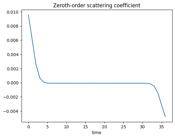
Question 10

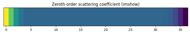
Plot the zeroth-order scattering coefficient, both in a 1d plot and also in an imshow plot as a vector.

Solution

order0 = np.where(meta['order'] == 0)

plt.plot(Sx[order0][0])
plt.title('Zeroth-order scattering coefficient')
plt.xlabel('time')
plt.show()

plt.figure(figsize=(10, 1))
plt.yticks([])
plt.imshow(Sx[order0], aspect='auto')
plt.title('Zeroth-order scattering coefficient (imshow)')
plt.show()

Question 11

Plot the first-order scattering coefficients, both in a 1d plot and also in an imshow plot as a matrix.

What is the name of the image plot?

Solution

import pandas as pd
order1 = np.where(meta['order'] == 1)
df = pd.DataFrame(Sx[order1].numpy().T)

df.plot(legend=False)
plt.ylabel("First-order scattering coefficients")
plt.xlabel("time")

Text(0.5, 0, 'time')

plt.imshow(Sx[order1].numpy(), aspect='auto')
plt.title('First-order scattering coefficients scalogram')

Text(0.5, 1.0, 'First-order scattering coefficients scalogram')

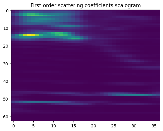
The name of the image plot is a scalogram, it shows the evolution of the signal in both time and (log) frequency.

Question 12

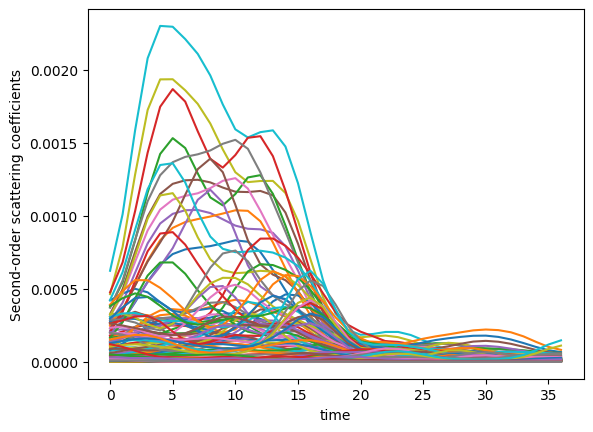
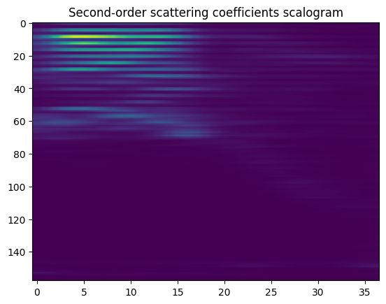
Plot the second-order scattering coefficients, both in a 1d plot and also in an imshow plot as a matrix.

Solution

order2 = np.where(meta['order'] == 2)
df = pd.DataFrame(Sx[order2].numpy().T)

df.plot(legend=False)
plt.ylabel("Second-order scattering coefficients")
plt.xlabel("time")

Text(0.5, 0, 'time')

plt.imshow(Sx[order2].numpy(), aspect='auto')
plt.title('Second-order scattering coefficients scalogram')

Text(0.5, 1.0, 'Second-order scattering coefficients scalogram')

Question 13

Using all the signals in the dataset, test the performance of a logistic regression classifier based on average wavelet scattering coefficients as features.

In the datset, index larger than 5 gets assigned to training set, and the rest to test set (i.e., a 90-10 split).

For the scattering transform, store the data in \(T=2^{13}\) samples (i.e., 8192), use \(J=8\) and \(Q=12\).

The features should be the wavelet scattering coefficients averaged over time, i.e., in the time dimension.

For the model, you can use:

model = Sequential(Linear(num_input, num_classes), LogSoftmax(dim=1))
optimizer = Adam(model.parameters())
criterion = NLLLoss()

Solution

from torch.nn import Linear, NLLLoss, LogSoftmax, Sequential
from torch.optim import Adam
from sklearn.metrics import confusion_matrix

use_cuda = torch.cuda.is_available()
device = torch.device("cuda" if use_cuda else "cpu")

device

device(type='cpu')

torch.manual_seed(42)

<torch._C.Generator at 0x11579f250>

T=2**13
J = 8
Q = 12

2**13, 2**8, 2**13/2**8

(8192, 256, 32.0)

# set a small number to avoid singular errors in logs.
log_eps=1e-16

path_dataset= info_dataset['path_dataset']
files=info_dataset['files']

x_all = torch.zeros(len(files), T, dtype=torch.float32, device=device)
y_all = torch.zeros(len(files), dtype=torch.int64, device=device)
subset = torch.zeros(len(files), dtype=torch.int64, device=device)

for k, f in enumerate(files):
    basename = f.split('.')[0]

    # Get label (0-9) of recording.
    y = int(basename.split('_')[0])

    # Index larger than 5 gets assigned to training set.
    if int(basename.split('_')[2]) >= 5:
        subset[k] = 0
    else:
        subset[k] = 1

    # Load the audio signal and normalize it.
    _, x = scipy.io.wavfile.read(os.path.join(path_dataset, f))
    x = np.asarray(x, dtype='float')
    x /= np.max(np.abs(x))

    # Convert from NumPy array to PyTorch Tensor.
    x = torch.from_numpy(x).to(device)

    # If it's too long, truncate it.
    if x.numel() > T:
        x = x[:T]

    # If it's too short, zero-pad it.
    start = (T - x.numel()) // 2

    x_all[k,start:start + x.numel()] = x
    y_all[k] = y

y_all

tensor([5, 3, 1,  ..., 1, 2, 4])

scattering = Scattering1D(J, T, Q).to(device) # the to device is important for GPU compatibility

x_all.shape

torch.Size([3000, 8192])

%%time
Sx_all = scattering(x_all) # can also use  scattering.forward(x_all)

CPU times: user 50.2 s, sys: 43.6 s, total: 1min 33s
Wall time: 35.1 s

Sx_all.shape

torch.Size([3000, 337, 32])

Our full batch of 3000 signals is now over 32 time points and each signal has a scattering transform with a hierarchy of 337 coefficients.

We remove the zeroth order coefficients as they dont carry useful information.

Sx_all = Sx_all[:,1:,:]

Let us log-normalize and regularize:

Sx_all = torch.log(torch.abs(Sx_all) + log_eps)

Average along the time dimension to get a time-shift invariant representation.

Sx_all = torch.mean(Sx_all, dim=-1)
Sx_all.shape

torch.Size([3000, 336])

8192/336

24.38095238095238

We now have a representation of our signals of dimension 336, rather than 8192.

We move on and train a logistic regression classifier. The output of this classifier (based on the logistic function, i.e., sigmoid) is a probablity for belonging to a class (i.e., 0, 1, .., 9).

Get the training data:

Sx_train, y_train = Sx_all[subset == 0], y_all[subset == 0]

y_train, y_train.shape

(tensor([5, 3, 1,  ..., 1, 2, 4]), torch.Size([2700]))

Remenber, our labels in y_train are just the spoken digits.

Standardized the data, to mean zero and unit variance:

mu_train = Sx_train.mean(dim=0)
std_train = Sx_train.std(dim=0)
Sx_train = (Sx_train - mu_train) / std_train

num_input = Sx_train.shape[-1]
num_classes = y_train.cpu().unique().numel()
model = Sequential(Linear(num_input, num_classes), LogSoftmax(dim=1))
optimizer = Adam(model.parameters())
criterion = NLLLoss()

model = model.to(device)
criterion = criterion.to(device)

# Number of signals to use in each gradient descent step (batch).
batch_size = 32
# Number of epochs.
num_epochs = 50
# Learning rate for Adam.
lr = 1e-4

nsamples = Sx_train.shape[0]
nbatches = nsamples // batch_size

nbatches,nsamples

(84, 2700)

Train the model:

for e in range(num_epochs):
    # Randomly permute the data. If necessary, transfer the permutation to the
    # GPU.
    perm = torch.randperm(nsamples, device=device)

    # For each batch, calculate the gradient with respect to the loss and take
    # one step.
    for i in range(nbatches):
        idx = perm[i * batch_size : (i+1) * batch_size]
        model.zero_grad()
        resp = model.forward(Sx_train[idx])
        loss = criterion(resp, y_train[idx])
        loss.backward()
        optimizer.step()

    # Calculate the response of the training data at the end of this epoch and
    # the average loss.
    resp = model.forward(Sx_train)
    avg_loss = criterion(resp, y_train)

    # Try predicting the classes of the signals in the training set and compute
    # the accuracy.
    y_hat = resp.argmax(dim=1)
    accuracy = (y_train == y_hat).float().mean()

    print('Epoch {}, average loss = {:1.3f}, accuracy = {:1.3f}'.format(
        e, avg_loss, accuracy))

Epoch 0, average loss = 1.401, accuracy = 0.571
Epoch 1, average loss = 1.134, accuracy = 0.689
Epoch 2, average loss = 0.972, accuracy = 0.766
Epoch 3, average loss = 0.867, accuracy = 0.780
Epoch 4, average loss = 0.779, accuracy = 0.817
Epoch 5, average loss = 0.716, accuracy = 0.835
Epoch 6, average loss = 0.670, accuracy = 0.846
Epoch 7, average loss = 0.640, accuracy = 0.830
Epoch 8, average loss = 0.615, accuracy = 0.843
Epoch 9, average loss = 0.569, accuracy = 0.856
Epoch 10, average loss = 0.549, accuracy = 0.863
Epoch 11, average loss = 0.526, accuracy = 0.871
Epoch 12, average loss = 0.510, accuracy = 0.870
Epoch 13, average loss = 0.490, accuracy = 0.879
Epoch 14, average loss = 0.479, accuracy = 0.874
Epoch 15, average loss = 0.467, accuracy = 0.878
Epoch 16, average loss = 0.446, accuracy = 0.889
Epoch 17, average loss = 0.438, accuracy = 0.892
Epoch 18, average loss = 0.435, accuracy = 0.886
Epoch 19, average loss = 0.428, accuracy = 0.886
Epoch 20, average loss = 0.428, accuracy = 0.878
Epoch 21, average loss = 0.403, accuracy = 0.894
Epoch 22, average loss = 0.403, accuracy = 0.893
Epoch 23, average loss = 0.393, accuracy = 0.894
Epoch 24, average loss = 0.389, accuracy = 0.895
Epoch 25, average loss = 0.381, accuracy = 0.896
Epoch 26, average loss = 0.375, accuracy = 0.897
Epoch 27, average loss = 0.368, accuracy = 0.902
Epoch 28, average loss = 0.364, accuracy = 0.902
Epoch 29, average loss = 0.357, accuracy = 0.907
Epoch 30, average loss = 0.353, accuracy = 0.904
Epoch 31, average loss = 0.340, accuracy = 0.911
Epoch 32, average loss = 0.342, accuracy = 0.913
Epoch 33, average loss = 0.344, accuracy = 0.903
Epoch 34, average loss = 0.330, accuracy = 0.906
Epoch 35, average loss = 0.336, accuracy = 0.906
Epoch 36, average loss = 0.327, accuracy = 0.914
Epoch 37, average loss = 0.321, accuracy = 0.916
Epoch 38, average loss = 0.325, accuracy = 0.909
Epoch 39, average loss = 0.320, accuracy = 0.915
Epoch 40, average loss = 0.331, accuracy = 0.906
Epoch 41, average loss = 0.306, accuracy = 0.918
Epoch 42, average loss = 0.319, accuracy = 0.907
Epoch 43, average loss = 0.310, accuracy = 0.912
Epoch 44, average loss = 0.302, accuracy = 0.922
Epoch 45, average loss = 0.304, accuracy = 0.911
Epoch 46, average loss = 0.298, accuracy = 0.917
Epoch 47, average loss = 0.292, accuracy = 0.922
Epoch 48, average loss = 0.295, accuracy = 0.918
Epoch 49, average loss = 0.293, accuracy = 0.915

Test the model on the test set:

Sx_test, y_test = Sx_all[subset == 1], y_all[subset == 1]
Sx_test = (Sx_test - mu_train) / std_train

response = model.forward(Sx_test)
avg_loss = criterion(response, y_test)

# Try predicting the labels of the signals in the test data and compute the
# accuracy.

y_hat = response.argmax(dim=1)
accuracy = (y_test == y_hat).float().mean()

print('TEST, average loss = {:1.3f}, accuracy = {:1.3f}'.format(
      avg_loss, accuracy))

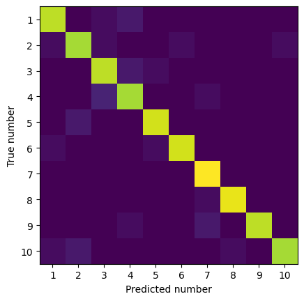
TEST, average loss = 0.289, accuracy = 0.913

Show the confusion matrix:

predicted_categories = y_hat.cpu().numpy()
actual_categories = y_test.cpu().numpy()

confusion = confusion_matrix(actual_categories, predicted_categories)
plt.figure()
plt.imshow(confusion)
tick_locs = np.arange(10)
ticks = ['{}'.format(i) for i in range(1, 11)]
plt.xticks(tick_locs, ticks)
plt.yticks(tick_locs, ticks)
plt.ylabel("True number")
plt.xlabel("Predicted number")
plt.show()